

Euler's Number
Euler's number, or number e, is the base of the natural logarithm: the unique number whose natural logarithm is equal to one. Euler’s number taps into fundamental laws of nature and the universe and is used extensively in Machine Learning algorithms.
Euler’s number is:
2.718...

ln(e) = 1
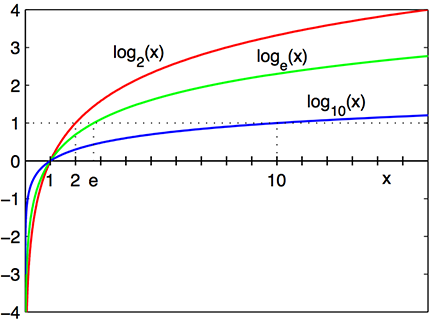
this shows how e log graphs fit with base 2 and 10
—-
By Richard F. Lyon - made myself, alt version of Logarithm plots.svg with better text, CC BY-SA 3.0, https://commons.wikimedia.org/w/index.php?curid=13257335
The Derivative of e to the Power of x
The function:
gives a curve at which the slope at any value x is also the value of y, which means the derivative is equal to the function itself, or:

this graph shows the slope of the function at various values of x
—-
https://www.wyzant.com/resources/lessons/math/calculus/derivative_proofs/e_to_the_x
Characteristics of e
e also has these important characteristics:
e is the base rate of growth shared by all continually growing processes
e shows up whenever systems grow exponentially and continuously, such as population, interest calculations and radioactive decay
every rate of growth can be considered a scaled version of e (unit growth, perfectly compounded)
e allows taking a simple growth rate where all change happens as the end of a finite period and find the impact of compound, continuous growth at infinitely smaller intervals
Compound Growth using e
Let's take a closer look at this last point, the impact of smaller intervals of compound growth calculation. Let:
F = the final future value after compound growth
I = the initial value before compound growth
r = rate of growth
t = time periods of time calculated
n = the number of compounding calculations within on period of time
The equation for calculating F is:
If we perform the calculation only once per period, then, n=1 and:
On the other extreme, if we perform compounding calculations continually letting n --> infinity, then:
So now we see how e fits into this equation. But how did it get there? To explore this, let's start with a simplified version of equation (1) above and let:
With these values, equation (1) becomes:
Now let's solve this equation for values of n. After n=10, we'll use a logarithmic scale and jump by a factor of 10 for each new calculation so we can see what happens with very large values of n:

notice how growth flattens when the value of the function reaches the value of e at around 2.718
In graph form, it looks like the chart below. Notice the jump between 10 and 100 as we move from a linear graph to a logarithmic graph for values of F:

after n=100, growth is relatively flat
What we see is that as the value of n approaches infinity, the value of F converges on the value of e: 2.7182820... This means that:
Another equation for calculating the value of e is:
An Example of Compound Growth using e
Let's look at an example of equation (1) when we let n --> infinity and have other values that are not equal to 1 for I, r, t:
equation (1) looks like this:
Combining the Rate of Growth and Time Periods using e
Using n --> infinity allows us to combine rate of growth and time periods calculated into one number. In the example above:
Deriving the Use of e in Compound Growth Equations
We haven't yet explained how we derived the following substitution in equation (1):
In other words, how did we simplify to using only e and rt as shown in equation (7)? Explaining it is a somewhat lengthy process, so we'll go through it in detailed steps...
Changing r/n to a Denominator
First, let's change r/n to a denominator using the algebraic rule of complex fraction inversion:
Applying the Power Rule to the Exponents
Next we're going to use the algebra power rule which says:
To do this, we'll first let:
and substitute it into our equation (8) so that::
Now we're going to introduce r into the exponent nt by adding it in as both a numerator and denominator that cancel each other out and rearranging the single fraction into two fractions, so that:
Now we'll apply the power rule from equation (9) with our new exponent values of x from equation (11) to get :
Next we'll replace x in equation (13) with the value from above:
Showing How e Enters our Equation
We still have to see how e enters this equation. To do this, within equation (14) let:
Within this equation, now look at:
Remember, we already know from equation (5) above that:
So equation (1) is basically the same as y except we're using n/r instead of just n. Now consider this:
Think about it, n/r might approach infinity at a somewhat slower pace than n, but it's still approaching infinity. So now we can say that for y from equation (15):
Using Backward Substitution to Show a Final Result
Now we can do backward substitutions through our sequence of equations to show a final result.
Combining equations (16) and (15) we have:
Combining equations (17) and (14) we have:
Combining equations (18) and (13) we have:
Combining equations (19) and (11) we have:
Combining equations (20) and (1) we have:
Which, finally, shows how we got to equation (3):